OLGA-Well-Kill A Poweful Tool for
Blowout and Kill Modeling
ABSTRACT
A new adaptation of a proven flow simulator is aiding blowout contingency planning. Most
important wells require a blowout contingency plan. Part of that plan includes relief well
intervention. The flow simulator distinguishes between workable and difficult intervention
schemes. It suggests any needed modifications in original well design and it makes crisis
management quicker, cheaper and more effective. This paper describes the power of using
this simulator for both surface and relief well hydraulic kill planning.
INTRODUCTION
Planning kill strategy for a 1989 underground blowout in the North Sea required
development of an improved flow simulator. The hydraulic kill simulator was based on the
industry-standard, two-phase pipe flow model, OLGA. After the project, the planning team
realized that they gained considerable advantage from using a transient two-phase flow
simulator for comparing various kill scenarios. Since that time the OLGA-WELL-KILL
simulator has been used successfully for a number of intervention design plans.
In the event of a major blowout, the speed at which rescue and intervention equipment and
personnel are mobilized is critical for the preservation of life, property and the
environment. The first priorities of these emergency operations are personnel evacuations,
oil spill containment and salvage of the reservoir, platform and well.
To respond quickly and efficiently to these emergencies, operators have devised and
supported emergency response plans with the necessary resources and infrastructure to
react immediately if required. Unfortunately, the only way to test the true effectiveness
of a response strategy is during an actual emergency. Only after the events can one
evaluate results and make modifications.
It is this reasoning, in the aftermath of recent major blowouts in the North Sea, that
operators and regulatory authorities are re-evaluating the status of emergency response
plans under their jurisdiction. Their purpose is to assure that lessons learned from these
events are documented and that all operators incorporate appropriate improvements into
their emergency procedures.
One component of this post evaluation process indicated that additional preparation for
regaining control of a blowing well is justified. Even though the probability of a blowout
is small, the consequences in safety, cost and pollution could be catastrophic. For these
reasons, "solving the problem" contingency plans are being added to the existing
emergency response plans. This effort will eventually include surface, subsea and relief
well intervention.
A primary objective of this contingency planning process is to evaluate the current level
of technology and operational expertise available for a blowout intervention operation.
Shortfalls can then be identified and appropriate action taken to reduce the deficiencies.
One problem identified early in this evaluation was the difficulty in analyzing heavy mud
hydraulic kills, in a two-phase blowout flow regime, with existing steady-state flow
models.
These models cannot easily evaluate the time transients of the kill process or deal with
complicated multiphase flow regimes, flow paths and interaction with the reservoir.
Example deficiencies include the inability to determine the rate at which mud will U-tube
from a relief well upon intersection with the blowout, the rate at which bottom hole
pressure will build up, or the kill volume required. Steady-state models cannot tell
whether gas will migrate during the pumping operation, how long peak HHP loads will be
required or how changing temperatures will effect overall design.
The ability to analyze hydraulic kill scenarios quickly and find their effect on the rest
of the intervention operation is critical to project success. A specialized need was
therefore identified for a multiphase, time-transient, flow simulator designed for easy
blowout kill analysis. This need was the driver that motivated the continued modification
of the pipeline code for well flow and kill simulations.
THE CONTINGENCY PLANNING OBJECTIVE
The successful planning and execution of a complicated blowout intervention operation
requires the careful coordination of several specialized technical disciplines. The
development of a strategy is an iterative process. It requires evaluating several
alternatives, analyzing risks and making tradeoffs, before reaching agreement between the
operator, partners, and regulatory authorities. These decisions carry substantial safety,
environmental and economic implications. The person or company responsible for the
intervention will perform with confidence if proper remedial contingency is performed
beforehand.
All blowouts and subsequent intervention techniques are
inherently different. This makes it impractical to cover all possibilities in specific
planning and execution procedures. However, a structured guideline, with examples, is
essential to avoid overlooking critical steps in the development of the final well control
strategy, where many decisions are made under stressful conditions.
The basic considerations include:
- Organizing a blowout intervention task force and project
management structure.
- Identifying critical equipment, personnel, contractors and
suppliers.
- Defining the blowout data acquisition requirements to
describe the situation accurately.
- Evaluating blowout intervention options (surface methods and
relief wells) and managing risks.
- Developing a general relief well and surface intervention
strategy.
- Developing specific relief well and surface intervention
strategies for hypothetical blowouts on critical structures and exploration wells.
- Evaluating circumstances that might make the intervention
project unusually difficult based on current technology and experience.
- Structuring for safety, documentation and technical audit
procedures.
RELIEF WELL PLANNING REVIEW
This paper illustrates the development of a single component of a relief well plan. The
following review shows how the flow simulator fits into that plan. The first step in this
process is to define the problem or "blowout scenario" accurately before
expensive solutions are planned. It is important to remember that the blowout scenario
controls the majority of the planning process. If the scenario is misinterpreted, the
blowout intervention plan may prove inadequate and dangerous. The first decision point is
to evaluate the hydraulic kill point, placing the depth, proximity, orientation and
position tolerance of the relief well intersection with the blowout wellbore. This most
critical step influences the entire relief well planning process and requires an iterative
analysis of all data as a system.
Once a point is chosen, two parallel planning paths must be
evaluated. One side considers a drilling design to place the relief well at the chosen
point considering all constraints. The other is to design the kill hydraulics and
associated pumping and special equipment to carry out the kill operation at the point
chosen. If both sides cannot achieve their goal with a reasonable degree of confidence,
then the kill point must be re-evaluated.
The new flow simulator evaluates the kill hydraulic portion of the overall relief well
design.
FLOW SIMULATOR DESCRIPTION
The well kill simulator, OLGA-WELL-KILL, stems from the dynamic two-phase pipe flow
simulator OLGA2. Development started in 1980 at Institutt for Energiteknikk (IFE) as a
project for Statoil, mainly aimed at simulation of terrain-induced slugging in pipelines.
From 1983, the development was carried out under the joint IFE/SINTEF Two-Phase Flow
Project with support from a group of oil companies. Emphasis was placed on verification of
the model against data from different experimental facilities, including the results from
the 8-in. diameter, 1000 m and 90 bar experimental flow loop at SINTEF. Several new
applications were added, such as gathering pipeline networks, compressors, heat
exchangers, separators, chokes, reservoir inflow, leaks and plugging. The model has been
used extensively and applied to a variety of situations such as pipeline design
simulations, pipeline shut-in, start up, and rupture studies.
 During the kill planning for the Saga Petroleum underground blowout (well
2/4-14 in 1989) 3-4, it was discovered that no suitable tool exists for dynamic estimation
of kill fluid volumes and times when a number of kill points and options are to be
evaluated. The more common approach of using conventional (steady state) tubing hydraulics
programs is time consuming and can be inaccurate, due to the need for a manual step-wise
approach. Applying the dynamic two-phase model OLGA to the problem improved modeling
capabilities, accuracy and turn-around time. The team could then compare different kill
options for both direct kill and relief well intervention.
During the kill planning for the Saga Petroleum underground blowout (well
2/4-14 in 1989) 3-4, it was discovered that no suitable tool exists for dynamic estimation
of kill fluid volumes and times when a number of kill points and options are to be
evaluated. The more common approach of using conventional (steady state) tubing hydraulics
programs is time consuming and can be inaccurate, due to the need for a manual step-wise
approach. Applying the dynamic two-phase model OLGA to the problem improved modeling
capabilities, accuracy and turn-around time. The team could then compare different kill
options for both direct kill and relief well intervention.
A Saga Petroleum research program has generated a new
simulator, OLGA-WELL-KILL, specially adapted to well flow kill applications. This
simulator has been used on actual blowouts and for contingency planning. Comment from this
work helped tailor features of the code toward the answers needed by the end users,
without compromising on the complexity or accuracy of the flow modeling process itself.
The model program now runs on portable computers.
During a blowout kill, up to six fluids can be present simultaneously in a well; reservoir
oil, gas and water, kill water, intermediate and final kill mud. Simulations handle this
by first simulating the dynamics of a liquid/gas biphasic flow regime, then comparing this
to a simulation using averaged properties in a light phase. The kill phase is then
introduced and a dynamic two-phase simulation performed until a steady state condition is
reached. Afterwards, the next phase can be introduced and the simulations can be restarted
at any time step.
Modeling is accomplished using a number of controllers set to contain the simulation
within the physical constraint of the real blowout.
 The controllers can, for example, be set on these parameters:
• Pump rate
• Pump horsepower
• Formation collapse pressure
• Casing burst pressure
• Surface injection pressure
• Bottom hole pressure (Min/Max)
The simulation modeling includes:
• Pump performance
• Non-Newtonian fluid flow (for mud)
• Fluid temperature and pressure response
• Inflow modeling (multiple if needed)
• Leaks (multiple if needed)
• Back pressure (outflow conditions)
• Several reservoir inflow models
• Variable reservoir pressure
• Path chokes (critical and sub-critical)
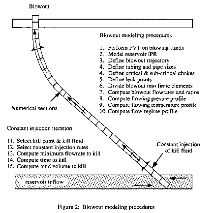
In practical use, the modeling is usually taken through a number of steps, starting with a
PVT fluid characterization of the reservoir fluids. The blowout is then modeled to match
all available data (Fig. 2). This can, for certain blowouts, provide a valuable exercise
in itself. It eliminates uncertainties. It is always much easier to solve the actual
problem at hand than to approach a well kill by trial and error.
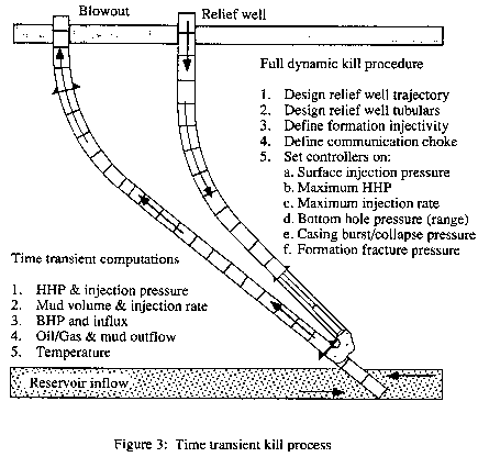
 The next step is to set up a constant rate kill
simulation to work out the range for the simulation of the actual dynamic kill. This is
also useful in evaluating allowance for losses between wells (for relief well kills) as
well as for the kill fluid density, and for velocity and pressures at critical points in
the blowout path. The fully dynamic simulations can then incorporate all the actual
constraints in the kill such as casing pressure ratings, fracture pressures, inflow
performance and reservoir pressure (dynamically versus time, if necessary), pumping plant
and mud properties (Fig. 3).
The next step is to set up a constant rate kill
simulation to work out the range for the simulation of the actual dynamic kill. This is
also useful in evaluating allowance for losses between wells (for relief well kills) as
well as for the kill fluid density, and for velocity and pressures at critical points in
the blowout path. The fully dynamic simulations can then incorporate all the actual
constraints in the kill such as casing pressure ratings, fracture pressures, inflow
performance and reservoir pressure (dynamically versus time, if necessary), pumping plant
and mud properties (Fig. 3).
The simulation yields an actual pump schedule vs. time (with rates and pressures at any
chosen point in the flow path). If needed, a number of sensitivities can be developed to
evaluate kill effectiveness during the actual pumping. This later step can often prove
useful when there are unknowns in the kill (such as communication between relief well and
blowout well, actual blowout flow path, or reservoir performance).
CASE HISTORY EXAMPLES
These examples are based on genuine contingency plans for hypothetical blowouts.
Simulations use actual well data.
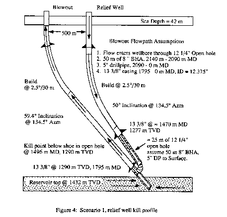
Scenario 1. A hypothetical relief well intervention was designed assuming a blowout to the
surface of a shallow gas well. In this case, 13 3/8-in. casing has been set at 1300 m TVD
with 12 1/4-in. open hole drilled through the reservoir to 1450 m TVD. The drillpipe is
sheared and dropped and the blowout flow path is up the annulus to the rig-floor.
 The kill point illustrated here assumes achieving
communication by direct intersection with the wellbore just below the 13 3/8-in. casing
shoe. This point is 140 m TVD above the top of the blowing zone. The reservoir is normally
pressured with a gradient of 1.08 sg EMW, the permeability is 400 md with a net thickness
of 30 m. The temperature is 54 �C, the fluid is dry gas and the fracture gradient is 2.46
psi/m (Fig 4).
The kill point illustrated here assumes achieving
communication by direct intersection with the wellbore just below the 13 3/8-in. casing
shoe. This point is 140 m TVD above the top of the blowing zone. The reservoir is normally
pressured with a gradient of 1.08 sg EMW, the permeability is 400 md with a net thickness
of 30 m. The temperature is 54 �C, the fluid is dry gas and the fracture gradient is 2.46
psi/m (Fig 4).
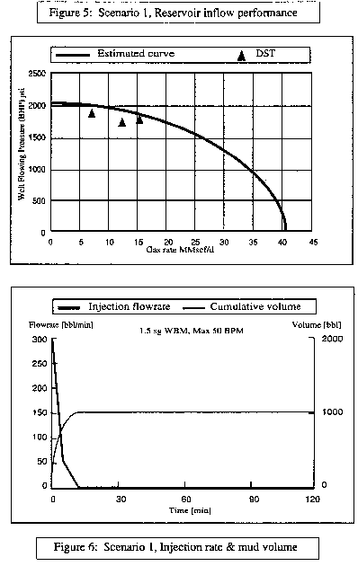
After performing a PVT analysis on the blowing gas, a
non-linear inflow performance (IPR) curve for the reservoir was developed. This relation
is important in an open flow gas blowout due to the potentially low flowing bottom hole
pressure. A linear PI will produce an unrealistically high blowout flow rate and
unnecessarily increase the kill hydraulic requirements (Fig. 5).
On the basis of on this IPR curve and the blowout flow path a steady state flow rate was
calculated at 41 MMscf/d of gas with no condensate. The flowing bottom hole pressure was
500 psi (static 2050 psi). The possibility of massive sand production and bridging or hole
collapse are strong possibilities under these conditions. For this exercise, flow remains
constant. Two kill fluids were evaluated, 1.14 sg water-based mud and seawater. The
constant injection of kill fluid into the well at the chosen kill point produced the
following results for mud then water:
| Pump rate (bpm) |
40 |
50 |
60 |
80 |
| Kill time (m) |
none |
32 |
14 |
7 |
| Volume (bbl) |
- |
1600 |
840 |
560 |
| Pump rate (bpm) |
100 |
110 |
120 |
130 |
| Kill time (m) |
none |
14 |
8 |
6 |
| Volume (bbl) |
- |
1540 |
960 |
780 |
These values give the minimum rates to control the well
dynamically, assuming no losses to the formation. The kill time and volumes indicated are
times at which the influx stops. Additional time and volumes will be required to flush gas
from the well. The seawater kill must be followed by mud with sufficient density to
control the static reservoir pressure.
The next iteration of the hydraulic planning process is to design a relief well to
intersect at the chosen kill point. Fig. 4 shows basic design.
The constant injection results provide the starting data
required for the controlled rate injection, where the full dynamic kill is simulated with
the relief well attached. For this paper only the mud kill will be discussed. The
controller limits for this simulation were set at 7500 psi injection pressure, 2500 psi
bottom hole pressure and a starting pump rate of 50 bpm. The simulator will adjust the
injection rate to stay within these limits after intersection. Figure 6 gives a double
"y" plot of flow rate and cumulative kill mud volume versus time. Observe that
immediately upon intersection with the blowout wellbore, mud U-tubes from the relief well
at rates approaching 280 bpm. This is due to the extreme pressure differential between the
relief well and the flowing blowout wellbore and the large diameter flow path. If the
injection rate at the surface could keep up with this suction rate at the intersection,
the well would be killed in just over 10 minutes with a cumulative mud volume of just over
1000 bbl.
 Since injection rates this high are not practical,
this information is valuable in evaluating the risks associated with this kill
alternative. For example, if a mechanical problem prevented immediate kill mud injection,
the relief well could reach a blowout situation in about 7 minutes.
Since injection rates this high are not practical,
this information is valuable in evaluating the risks associated with this kill
alternative. For example, if a mechanical problem prevented immediate kill mud injection,
the relief well could reach a blowout situation in about 7 minutes.
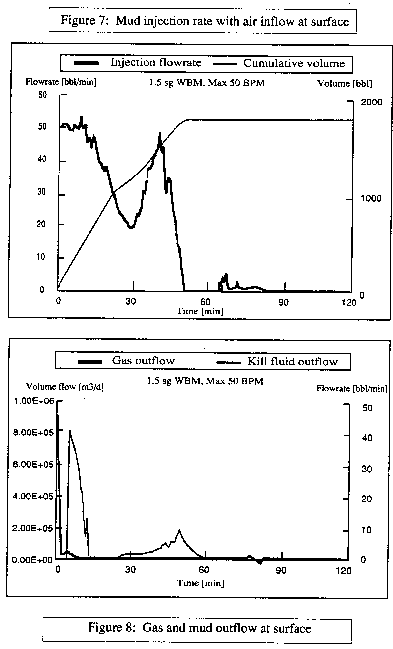
Figure 7 shows a double "y" plot of flow rate and cumulative kill mud volume
versus time with a maximum injection rate of 50 bpm at the surface. In this case the
difference between the surface injection of 50 bpm and the bottom hole suction is replaced
by air. This scenario yields a kill time of �50 minutes and a cumulative volume of �1800
bbl. The hump in the flow rate curve at 40 minutes is caused by the air circulating around
the blowing well.
Figure 8 shows a double "y" plot of gas outflow and kill mud outflow versus
time. The kill fluid outflow, between 5 and 10 minutes corresponds to the kill pumping
volume. However, the outflow indicated between 25 and 60 minutes occurs after the pumps
have stopped. Further evaluation of the two-phase fluid distribution in the blowout
wellbore indicated that the kill mud was falling to the low side of the 60� inclination
hole while pushing the gas to the high side and trapping a gas bubble below the
intersection point. This bubble migrated to the surface after the pumps were stopped and
ejected a substantial volume of mud from the blowout well.
If this reduced mud column had been insufficient to hold the reservoir pressure, the well
would have started flowing again. This simulation demonstrates the need to continue
circulating at a low rate for several blowout hole volumes after the well is statically
dead.
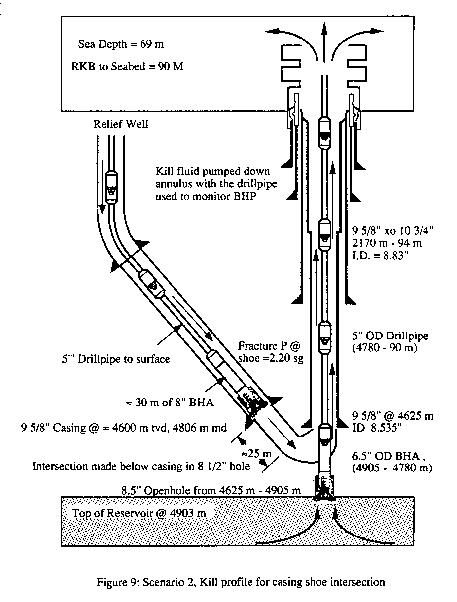
Scenario 2. In this example a hypothetical relief well intervention was designed for a
deep high pressure, high temperature exploration well. In this case, 9 5/8-in. casing has
been set vertical at 4600 m with a leak-off test of 2.20 sg. The 8 1/2-in. hole
intersected the top of a hydrocarbon pressure compartment at 4900 m TVD, 100 m higher than
predicted and is penetrated by 2 m. The 5-in. drillpipe is sheared and dropped to the
bottom. The flow path is up the annulus, with no restrictions, to the seabed.
Two kill points were evaluated, one at the 9 5/8 in. shoe,
280 m above the reservoir and another at the reservoir top. Both kill points assume
direct communication through open hole. The position tolerance required at intersection is
+/- 1m. Data on the sandstone reservoir is estimated as:
| PI (estimate) |
30 Sm3/day/bar |
| Depth |
4900 m TVD |
| Permeability |
10 md |
| Pressure (TD) |
1030 Bar (2.14 sg) |
| BHT |
180 C |
| Fluid |
Gas/cond. |
| GCR |
500 Sm3/Sm3 |
| Bottom Hole Pressure |
750 bar |
| Gas Rate |
2 MMSm3/d |
| Condensate Rate |
4000 Sm3/d |
The 9 5/8-in. intersection can be drilled much quicker and
with a higher probability of achieving the +/- 1m placement criteria. However, there is
risk the kill operation may exceed the fracture pressure at this depth. The deeper kill
point has hydraulic and fracture strength advantages. However, the high bottom hole
temperatures and depth will cause serious directional drilling control problems thus
increasing the risk that the well might miss +/- 1m intersection. The simulator was used
to determine if the off-bottom kill has acceptable risk with respect to the kill
hydraulics (Fig 9).
Based on the assumed inflow performance of the reservoir, the hydrocarbon composition, and
the flow path, the following blowout rates were computed:
Two different kill fluids were evaluated, 2.2 sg
water-based mud and seawater. The minimum flow rate for a seawater kill was 100 bpm at the
shoe and 90 bpm at TD. Both of these rates would require unrealistically large pumping
plants and were not considered further.
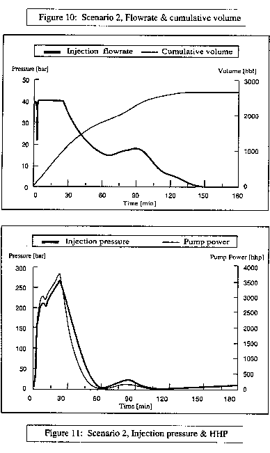
The constant injection iteration at the shoe kill point
required a minimum flow rate of 35 bpm to a achieve a kill in 64 minutes using 2240 bbl of
mud. A 40 bpm rate reduced the kill time to 27 minutes and a corresponding 1080 bbl of
mud. A 35 bpm injection rate at the bit would kill the well in 34 minutes using 1190 bbl
of mud. Initial injection rates of 40 bpm for the shoe intersection and 35 bpm for the bit
intersection were chosen for the full transient simulations with the relief well attached.
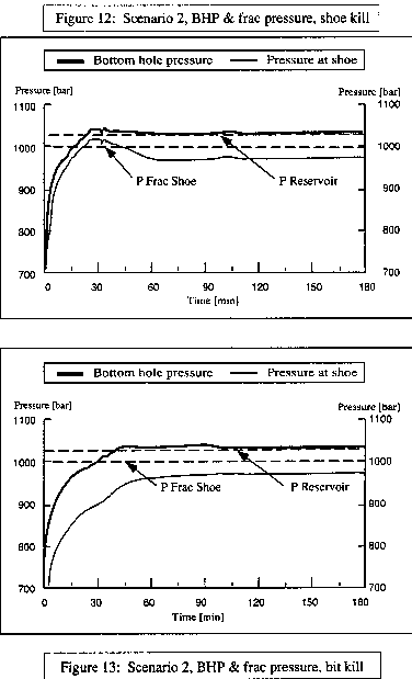
 Figures 10-12 illustrate double "y" plots
of mud injection rate and cumulative mud volume, pump power and injection pressure, and
bottom hole pressure and pressure at the shoe respectively, for the casing shoe kill
scenario. Figure 12 shows that fracture pressure at the shoe is exceeded slightly just as
the gas below the kill point is bullheaded back into the formation. Figure 13 illustrates
the bottomhole pressure and casing shoe pressure for the bit kill scenario. This plot
shows pressure remains below fracture gradient for this intersection point.
Figures 10-12 illustrate double "y" plots
of mud injection rate and cumulative mud volume, pump power and injection pressure, and
bottom hole pressure and pressure at the shoe respectively, for the casing shoe kill
scenario. Figure 12 shows that fracture pressure at the shoe is exceeded slightly just as
the gas below the kill point is bullheaded back into the formation. Figure 13 illustrates
the bottomhole pressure and casing shoe pressure for the bit kill scenario. This plot
shows pressure remains below fracture gradient for this intersection point.
These simulations further substantiate the difficulty in
planning a kill for a deep, pressured blowout. Deep intersection can handle kill
hydraulics, but risks intersection failure. Casing shoe intersection is easier but pumping
will fracture the rock. Further investigation would be required on the rate and linearity
of the loss to determine if the hydraulics at this kill point are too risky to attempt.
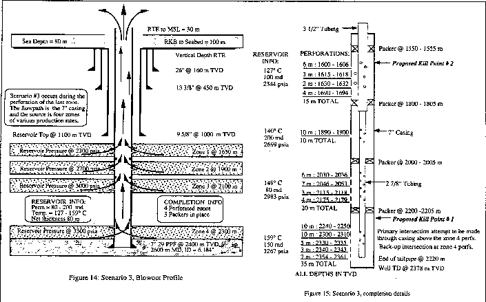
Scenario 3. In this example a hypothetical relief well intervention was designed for a
normally pressured gas condensate blowout during completion. In this case, 7-in.
production casing has been set through four producing reservoirs, each with different
hydrocarbon compositions, temperatures and IPR curves. A single 3 1/2-in. completion
string is used. Each zone has been perforated and isolated from others by three production
packers. Fluids from each zone mingle in the production tubing. The blowout is assumed
after perforating the last zone. All zones are flowing to the surface with only the
wireline in the casing (Fig. 14).
 This scenerio evaluates kill points at
the top of the lower set of perforations in zone 4 at 2200 m, and at the top of the first
set of perforation in zone 1 at 1600 m. The extreme temperature gradient of this well, 1.8
�C/30 m, will make an intersection at 2200 m complicated due to directional drilling
limitations at 160 �C. Therefore an intersection at 1600 m is attractive if the well can
be controlled at this depth without exceeding the fracture gradient. The hydraulics at
this depth are complicated by the multiple flowing zones with different characteristics
and pressures. The simulator, however, can handle these multiple zones easily (Fig. 15).
This scenerio evaluates kill points at
the top of the lower set of perforations in zone 4 at 2200 m, and at the top of the first
set of perforation in zone 1 at 1600 m. The extreme temperature gradient of this well, 1.8
�C/30 m, will make an intersection at 2200 m complicated due to directional drilling
limitations at 160 �C. Therefore an intersection at 1600 m is attractive if the well can
be controlled at this depth without exceeding the fracture gradient. The hydraulics at
this depth are complicated by the multiple flowing zones with different characteristics
and pressures. The simulator, however, can handle these multiple zones easily (Fig. 15).
Based on reservoir and fluid property characteristics the blowout rates for each zone are:
| Zone |
Reservoir P [psi] |
Flowing P [psi] |
GasRate
MMscf/d |
| 1 |
2300 |
2100 |
20 |
| 2 |
2700 |
2300 |
60 |
| 3 |
3000 |
2350 |
40 |
| 4 |
3300 |
2400 |
80 |
| Total |
|
|
200 |
Two kill fluids were evaluated, 9.5 ppg water-based mud,
and seawater, for both intersection points. The steady injection rate iteration indicated
that a minimum of 35 and 45 bpm of mud and 40 and 50 bpm of seawater would be required to
kill the well at zone 4 and zone 1 respectively. Two relief wells were planned based on
the intersection points. Full dynamic simulations were based on these initial injection
rates with the relief well attached. Table 1 summarizes results.
The well can be controlled from an intersection in zone 1
without exceeding the fracture gradient and without excess pumping requirements.
Scenario 4. This example is based on a gas and water
blowout during a workover with a snubbing unit. While fishing 2 3/8-in. tubing a hole
developed in the production casing which caused failures in the 9 5/8-in. and the 13
3/8-in. casing.
It burst just below the wellhead. The well was soon brought under partial control with the
flow manifolded to allow pressure to bleed off the annuli and to separate the gas and
water.
 The mechanical situation downhole was
complicated, with considerable uncertainty about the flow path from the reservoir to the
surface. At the time the problem occurred the tubing had been removed to 4500 ft just
above a nipple. It was assumed this nipple was obstructing the tubing ID and a 270 ft, 4
1/2-in. OD wash-pipe assembly with an outside cutter had consequently been run in the
hole, swallowing the tubing. There was no pressure seal between the tubing and wash pipe
but the tolerances between the 5 1/2-in. production casing and the 4.5-in. OD of the wash
pipe provided a tight restriction for flow. Noise logs run through the work string
indicated there were holes in the casing at 4500 and 1600 ft MD. This allowed a leak into
a 4 Darcy permeability water sand if shut in at the surface. A proposal was made to pump
18 ppg mud down the work string at a maximum rate in an attempt to stop the flow. However,
due to the unknown flow path and known holes in the casing, there was some risk that the
mud flow might increase the hole size in the casing and cause the blowout to broach to the
surface.
The mechanical situation downhole was
complicated, with considerable uncertainty about the flow path from the reservoir to the
surface. At the time the problem occurred the tubing had been removed to 4500 ft just
above a nipple. It was assumed this nipple was obstructing the tubing ID and a 270 ft, 4
1/2-in. OD wash-pipe assembly with an outside cutter had consequently been run in the
hole, swallowing the tubing. There was no pressure seal between the tubing and wash pipe
but the tolerances between the 5 1/2-in. production casing and the 4.5-in. OD of the wash
pipe provided a tight restriction for flow. Noise logs run through the work string
indicated there were holes in the casing at 4500 and 1600 ft MD. This allowed a leak into
a 4 Darcy permeability water sand if shut in at the surface. A proposal was made to pump
18 ppg mud down the work string at a maximum rate in an attempt to stop the flow. However,
due to the unknown flow path and known holes in the casing, there was some risk that the
mud flow might increase the hole size in the casing and cause the blowout to broach to the
surface.
The simulator evaluated some of these risks. Various flow
paths from the reservoir to the surface were simulated and compared to the measured flow
at the surface. It was originally suspected the flow path was behind the casing from the
reservoir. Simulation results, however, indicated that the gas was more likely flowing up
the 2 3/8-in. tubing from the reservoir, around the wash pipe and up the 5 1/2 by 2
7/8-in. annulus to the surface. This simulation most closely matched flow measured at
surface. A pump test was also simulated by injecting fresh water down the work string at
3.5 bpm, mixing with the gas and saltwater flow in the wash pipe. This was compared with
the assumed flow path and the changing outflow conditions. These results also supported
the model-predicted flow path (Fig. 16). Confident of the flow path, a dynamic kill
simulation was made using the 18 ppg mud pumped down the work string at 3 bpm.
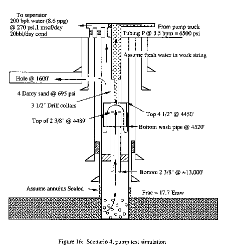 These simulations indicated the wash pipe would
create sufficient friction pressure during pumping to bullhead the gas and water back to
the reservoir from 4400 ft to 10,900 ft. The inflow would be stopped in 25 minutes, with
175 minutes required to flush all the gas and water from the well. The injection rate was
reduced from 3 bpm to 1 bpm after 60 minutes. These simulations were performed assuming a
hole in the casing at 1600 ft with a back pressure of 695 psi.
These simulations indicated the wash pipe would
create sufficient friction pressure during pumping to bullhead the gas and water back to
the reservoir from 4400 ft to 10,900 ft. The inflow would be stopped in 25 minutes, with
175 minutes required to flush all the gas and water from the well. The injection rate was
reduced from 3 bpm to 1 bpm after 60 minutes. These simulations were performed assuming a
hole in the casing at 1600 ft with a back pressure of 695 psi.
SUMMARY AND CONCLUSIONS
A new computer program can simulate multiphase flow in a blowout and a relief well. The
simulator comes from proven pipeline flow models. We have used the simulator to design
kills for factual blowouts. More importantly, we believe the simulator provides a valuable
tool for contingency planning. Results are both quicker and more accurate than previous
methods.
The OLGA-WELL-KILL simulator can find a workable relief-well strategy before drilling
begins and it can point out design changes to make contingent operations safer and
cheaper.
The simulator adapts existing pipeline technology
(developed with substantial funding) to hydraulic kill applications. The core code, which
acts as the simulator engine, was extensively tested over the last 10 years and remains
unchanged. Modifications allow quick analysis of transient multiphase flow regimes under a
variety of complicated blowout and kill scenarios. Analysis can be made by pumping either
from a relief well or directly into the blowout.
Experience and research have shown that the hydraulic kill
design is a major driver in the overall intervention project, particularly in the case of
relief well control. This capability to simulate blowout flow, temperature, kill fluid
weights and volumes, hydraulic horsepower, pressures and other related parameters all with
respect to time and at any point in the well, has not been available to the industry
before.
The four examples here illustrate some capabilities. Other
applications include:
• Kill with different mud densities in the well
• Partial losses during kill
• Multiple blowout paths, cross flows and leaks
• Multiple relief wells pumping at different rates
• Underground blowouts from a drilling rig
• Simultaneous bull heading and dynamic kill
• Off bottom or momentum kills
• Shallow gas blowouts
• Horizontal well flow analysis
• Slugging in long reach production wells
• Rates required to circulate out a kick in high-angle or
horizontal wells
• Alternating gas and water injection
• Sensitivity analysis by varying parameters
Soft intangibles are a hard sell. But the safety, environmental and economic risk of a
major blowout in today's world are too high to continue the historical
'react-if-it-occurs' approach. The technology for successful intervention has, in most
cases, matured to adequate levels, but every well requires adaptations. These adaptations
are best evaluated before an emergency occurs. A solid contingency plan makes any well
safer.
NOMENCLATURE
bha = bottom hole assembly
bht = bottom hole temperature
bpm = barrels per minute
EMW = Equivilent mud weight
GCR = gas condensate ratio
GOR = gas oil ratio
hhp = hydraulic horsepower
ID = inner diameter
IPR = inflow performance relation
m = meters
MD = measured depth
OD = outer diameter
PI = linear productivity index
PVT = pressure, volume, temperature
rte = rotary table elevation
sg = specific gravity, water = 1, air = 1
tvd = true vertical depth
REFERENCES
1. Wright, J.W.: "Blowout Intervention Preparedness Through Relief
Well Contingency Planning," Presented at the IADC European Well Control Conference,
June 11-13, 1991, Stavanger, Norway.
2. Bendiksen, K., Malnes, D., Moe, R. and Nuland, S.: "The Dynamic
Two-Fluid Model OLGA: Theory and Application," SPE Production Engineering, May 1991.
3. Leraand, F., Wright, J., Zachary, M., and Thompson, B.:
"Relief Well Planning and Drilling for a North Sea Underground Blowout," JPT,
March, 1992, p.266.
4. Rygg, O.B. and Gilhus, T.: "Use of Two-Phase Pipe Flow Simulator
in Blow-out Kill Planning," SPE 20433 presented at the 65th Annual Conference in New
Orleans, Oct. 23-26, 1990.
5. Blount, E. M. and Soeiinah E.: "Dynamic Kill: Controlling Wild
Wells a New Way, "World Oil, October, 1981, p. 109-126.